High-Fidelity, Compact, Real-Time Rendering of the Aalto Campus

February 23, 2026

Overview

Welcome to my 3D model of Aalto University, where I spent my master’s studies.but mostly hanging out and tinkering on different projects with my friends. :)

This project is made possible by recent advances in Gaussian Splatting. The scene was captured with DJI Mini 5 Pro, aligned in COLMAP, trained in gsplat with MCMC, compressed by SOGS, and rendered in PlayCanvas.

In this post, I’ll cover the main stages of the pipeline and walk through some of the practical implementation details. The Web viewer code is in hoanhle/3d, and Gaussian Splatting training code is in hoanhle/gsplat. Dataset can be downloaded from here.

Structure-from-Motion (SfM)

⊕
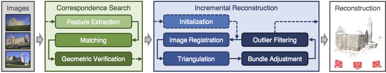
Incremental Structure-from-Motion pipeline

Structure-from-Motion (SfM) estimates a scene’s 3D structure and each camera’s intrinsic and extrinsic parameters from a set of overlapping 2D images. It is now a standard preprocessing step in modern view-synthesis pipelines. For Neural Radiance Fields (NeRF), SfM provides the camera poses required for training. For 3D Gaussian Splatting, SfM provides both camera poses and an initial sparse point cloud used to initialize the Gaussians.

Among practical SfM implementations, COLMAPI used COLMAP because it is the pipeline I am most familiar with and have end-to-end technical understanding of, but alternatives such as RealityCapture can also be used. has become the de facto standard. It is an open-source system with both incremental and global reconstruction pipelines, and it integrates naturally with dense multi-view stereo for robust and accurate reconstructions. The computational pipeline starts with feature detection and extraction, followed by matching, geometric verification, and finally structure and motion reconstruction to obtain these parameters.

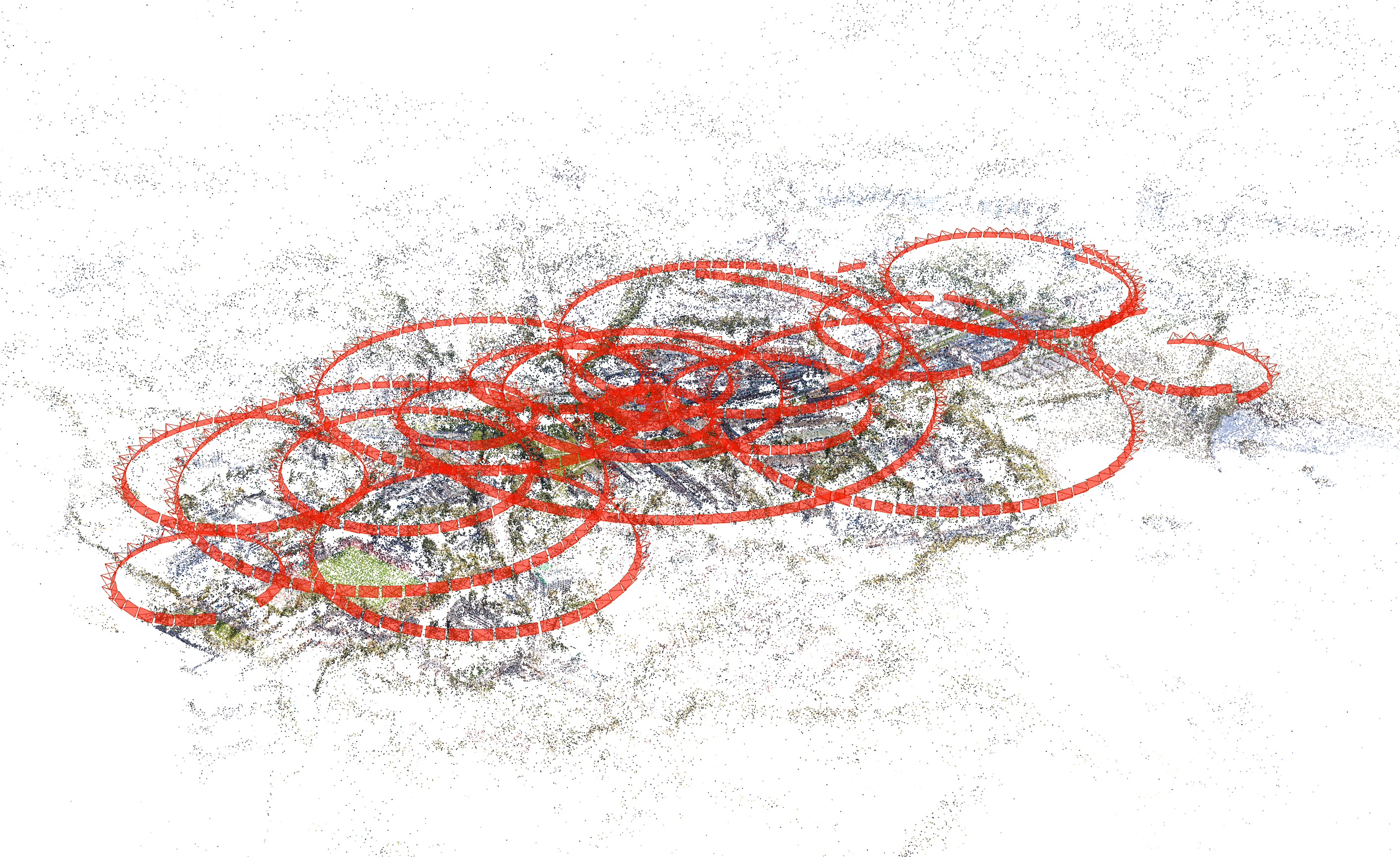
For this project, I captured the data with a DJI Mini 5 ProI literally bought my first drone for this project after playing around with my friend’s drone. DJI Mini 5 Pro is a good starter drone for this kind of project, especially with Circle QuickShot mode enabled., filtered out duplicated shots, merged the selected clips with ffmpeg, and then extracted PNG frames by sampling one frame every 300 frames. I then ran COLMAP on those images and obtained the reconstruction below.

3D Gaussian Splatting

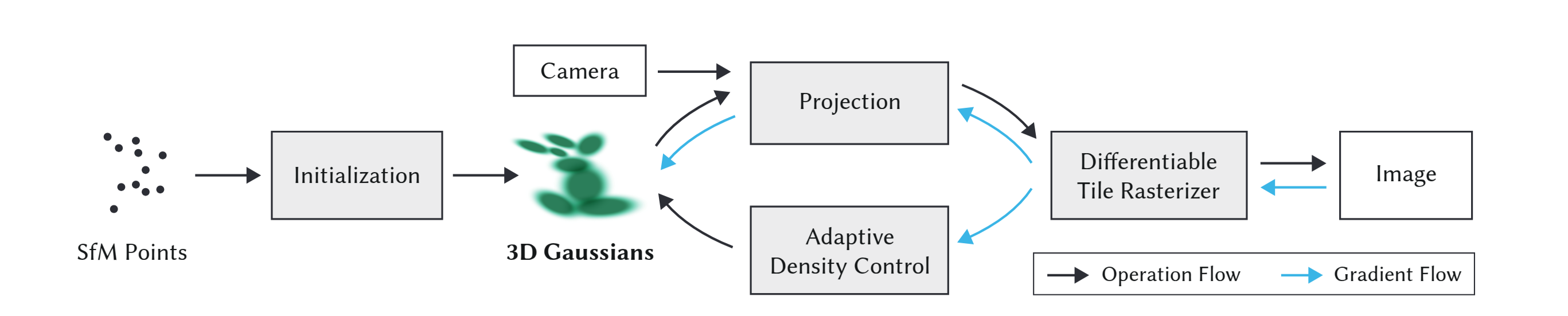
Given the calibrated cameras and sparse point cloud from SfM, we initialize the scene with a set of 3D Gaussians, each parameterized by mean (position), covariance (shape/orientation), opacity alpha, and view-dependent color represented with spherical harmonics (SH). The rendering pipeline projects these Gaussians onto the image plane as 2D ellipses, evaluates their color and opacity, and alpha-composites them in visibiliy order using a tile-based rasterizer. Training alternates between optimizing Gaussian parameters end to end against ground truth images and adaptive density control (splitting, cloning, and pruning). I will walk through each stage below.

Initialization

Kerbl et al. models the scene as a set of 3D Gaussians, defined as

where $\mu$ is the mean, $\Sigma$ is the covariance matrix. To ensure $\Sigma$ remains positive semi-definite during gradient-based optimization, it is decomposed into rotation matrix $R \in SO(3)$ and scale diagonal matrix $S \in R^{3x3}$ to represent the covariance matrix as $\Sigma = R SS^T R^T$. In practice, R and S are represented as a quaternion $q \in R^4$ and a vector $s \in R^3$.

During initialization, each point in the sparse point cloud seeds one 3D Gaussian, the mean centered at that point’s position, with its initial scale as the mean distance to its nearest neighbors. RGB colors are converted into zeroth-order SH coefficients, with higher-order bands set to 0. Quaternions are randomly initialized and opacities are set to a uniform default. All parameters are differentiable and optimized jointly during training. Pseudo code to initialize the Gaussians is below.

# pseudo-code, not meant to be used directly
def initialize_splats(points_xyz, points_rgb, cfg):
    points = tensor(points_xyz).float()                # [N, 3]
    rgbs = tensor(points_rgb / 255.0).float()          # [N, 3]

    # scale ~= average distance to the 3 nearest neighbors
    dist2_avg = mean(knn(points, k=4)[:, 1:] ** 2, dim=-1)  # [N], skip self
    dist_avg = sqrt(dist2_avg)

    # use log scale to avoid negative values
    scales = log(dist_avg * cfg.init_scale).unsqueeze(-1).repeat(1, 3)  # [N, 3]

    N = points.shape[0]

    params = {
        "means": Parameter(points),
        "scales": Parameter(scales),
        "quats": Parameter(rand(N, 4)),
        "opacities": Parameter(logit(full((N,), cfg.init_opacity))),
    }

    colors = zeros(N, (cfg.sh_degree + 1) ** 2, 3)  # [N, K, 3]
    colors[:, 0, :] = rgb_to_sh(rgbs)
    params["sh0"] = Parameter(colors[:, :1, :])
    params["shN"] = Parameter(colors[:, 1:, :])

    splats = ParameterDict(params).to(cfg.device)
    return splats

Projection

Within the 3DGS framework, each 3D Gaussian first needs to be projected to the camera image plane in order to determine its contribution to the individual pixels. To do this, the coveriance matrix $\Sigma^{\prime}$ for a projected Gaussian is computed as

where $W$ transforms the 3D Gaussian from world space to camera space, and $J$ is the Jacobian of the affine approximation of the projective transformation.Perspective projection is nonlinear because of depth division. To make it linear, 3DGS uses the first order Taylor approximation $f(\mu+\delta) \approx f(\mu) + J\delta$ where J (Jacobian) is the matrix of first partial derivatives, $J_{ij}=\partial f_i/\partial x_j$, evaluated at the Gaussian mean. This gives the local affine approximation. Let $\delta = X-\mu$ and $\Sigma = \mathbb{E}[\delta\delta^T]$. Then with first-order projection $Y=f(X)\approx f(\mu)+J\delta$, we get $\Sigma_Y=\operatorname{Cov}(Y)\approx \mathbb{E}[(J\delta)(J\delta)^T] $$=J\mathbb{E}[\delta\delta^T]J^T=J\Sigma J^T$.

For a pinhole camera with $ u = f_x X/Z + c_x,\quad v = f_y Y/Z + c_y $, the Jacobian with respect to camera-space coordinates $(X,Y,Z)$ is $J= \begin{bmatrix} \frac{f_x}{Z} & 0 & -\frac{f_x X}{Z^2} \\ 0 & \frac{f_y}{Z} & -\frac{f_y Y}{Z^2} \end{bmatrix},$ evaluated at the Gaussian mean in camera space.

# pseudo-code pytorch implementation, actual implementation is usually in CUDA for speed.
def project_pinhole(means: torch.Tensor, covars: torch.Tensor, Ks: torch.Tensor, width: int, height: int) -> Tuple[torch.Tensor, torch.Tensor]:
    """Project Gaussians' means and covariances from camera coordinate system to image coordinate system."""
    tx, ty, tz = torch.unbind(means, dim=-1)

    # NOTE: could add guard for zero division by tz using
    # tz = tz.clamp(min=1e-6)
    tz2 = tz**2

    fx = Ks[..., 0, 0, None]
    fy = Ks[..., 1, 1, None]
    cx = Ks[..., 0, 2, None]
    cy = Ks[..., 1, 2, None]
    tan_fovx = 0.5 * width / fx
    tan_fovy = 0.5 * height / fy

    # NOTE: empircally set safety margin
    lim_x_pos = (width - cx) / fx + 0.3 * tan_fovx
    lim_x_neg = cx / fx + 0.3 * tan_fovx
    lim_y_pos = (height - cy) / fy + 0.3 * tan_fovy
    lim_y_neg = cy / fy + 0.3 * tan_fovy
    tx = tz * torch.clamp(tx / tz, min=-lim_x_neg, max=lim_x_pos)
    ty = tz * torch.clamp(ty / tz, min=-lim_y_neg, max=lim_y_pos)

    O = torch.zeros_like(tz)
    J = torch.stack(
        [fx / tz, O, -fx * tx / tz2, O, fy / tz, -fy * ty / tz2], dim=-1
    ).reshape(means.shape[:-1] + (2, 3))

    # See equation (5) in https://arxiv.org/pdf/2308.04079
    cov2d = torch.einsum("...ij,...jk,...kl->...il", J, covars, J.transpose(-1, -2))
    
    # u = fx * x / z + cx
    # v = fy * y / z + cy
    means2d = torch.einsum("...ij,...nj->...ni", Ks[..., :2, :3], means) # [..., C, N, 2]
    means2d = means2d / tz[..., None] # [..., C, N, 2]
    return means2d, cov2d

Differentiable Tile Rasterizer

To have fast overall rendering performance, 3DGS uses a tile-based rasterizer. The screen is split into 16$\times$16 tiles, and each 3D Gaussian is culled against the camera frustum and then against individual tiles. A Gaussian that overlaps multiple tiles is instantiated once per tile, and each instance receives a sort key that packs the tile ID and view-space depth into a single integer. All keys are sorted together with a fast GPU radix sort, producing depth-ordered, per-tile list of Gaussians. For each tile, the first and last index are recorded into that sorted list, so every tile knows exactly which Gaussians contribute to it.

3DGS launches one CUDA thread block per tile. The block collaboratively loads Gaussians from global into shared memory and then each thread (one per pixel) alpha-composites color front-to-back. A pixel thread stops early once its accumulated opacity saturates (i.e., $\alpha \to 1$). The final pixel color is

where $c_i$ is the color of each point and $\alpha_i$ is the product of the learned per-Gaussian opacity and the 2D Gaussian evaluated at the pixel center.

Below is pseudocode for the rasterizer. For a deeper understanding, I recommend reading the CUDA rasterizer in the official diff-gaussian-rasterization repository. It is the main computational bottleneck and therefore critical to optimization efficiency.

# pseudo-code, mirrors Algorithm 2 from 3D Gaussian Splatting
def rasterize(w, h, means_ws, covars_ws, colors, opacities, view):
    # 1) cull and project
    visible = cull_gaussian(means_ws, covars_ws, view)  # full camera frustum
    means_ss, covars_ss, depths = screenspace_gaussians(
        means_ws[visible], covars_ws[visible], view
    )

    # 2) tile binning with global key sort
    tiles = create_tiles(w, h, tile_size=16)
    indices, keys = duplicate_with_keys(means_ss, covars_ss, depths, tiles)
    indices, keys = sort_by_keys(indices, keys)  # key = (tile_id, depth)
    tile_ranges = identify_tile_ranges(tiles, keys)

    # 3) rasterize per tile, per pixel, front-to-back alpha compositing
    image = zeros((h, w, 3))
    alpha = zeros((h, w))

    for tile in tiles:
        begin, end = get_tile_range(tile_ranges, tile)
        for px in pixels_in_tile(tile):
            T = 1.0  # residual transmittance
            rgb = vec3(0.0)
            for k in range(begin, end):
                g = indices[k]
                w_g = gaussian_2d_weight(px, means_ss[g], covars_ss[g])
                a = clamp(opacities[g] * w_g, 0.0, 0.99)
                alpha_next = 1.0 - T * (1.0 - a)
                if alpha_next > 0.9999:  # stop before exceeding opacity cap
                    break
                rgb += T * a * colors[g]
                T *= (1.0 - a)

            image[px] = rgb
            alpha[px] = 1.0 - T

    return image, alpha

Optimization

After rasterization, we compare the rendered image $\hat{I}$ with the ground-truth image $I$ and optimize using Stochastic Gradient Descent (SGD) with the loss function

Adaptive Density Control

As discussed in Initialization, 3DGS starts with an initial set of sparse points from SfM. However, due to the ambiguities of 3D-to-2D projection, some geometry may be placed incorrectly. The optimization therefore needs to create, destroy, or move geometry as necessary. To this end, 3DGS employs adaptive density control: Gaussians whose opacity falls below a threshold are pruned, while those with large view-space positional gradients (e.g: $0.0002$), a heuristic indicating either a region with missing geometric features (“under-reconstruction”) or regions where Gaussians cover large areas in the scene (“over-reconstruction”), are densified.

Small Gaussians in under-reconstructed regions are cloned: an identical copy is created and displaced along the positional gradient to cover the missing geometry. Large Gaussians in high-variance regions are instead split into two smaller ones, each with its scale reduced by a factor of $\phi = 1.6$ (determined experimentally), and their positions initialized by sampling from the original Gaussian as a probability density function.

After an optimization warm-up, 3DGS densifies every 100 iterations. It also resets opacity to near zero every 3000 iterations, allowing opacity to recover only where it is truly needed while enabling the culling of near-transparent Gaussians as described above and helping reduce floater artifacts.

Running 3DGS on our dataset

Now, with an overview understanding of the 3DGS pipeline, let’s run it on our dataset, using gsplat’s implementation. I stored my default config inside my fork.

python3 simple_trainer.py default \
  --data_dir ./data/aalto/ \
  --data-factor 2 \
  --result-dir results/aalto/naive \
  --save-ply

The results look pretty good, with examples below (left is ground-truth, right is rendered).

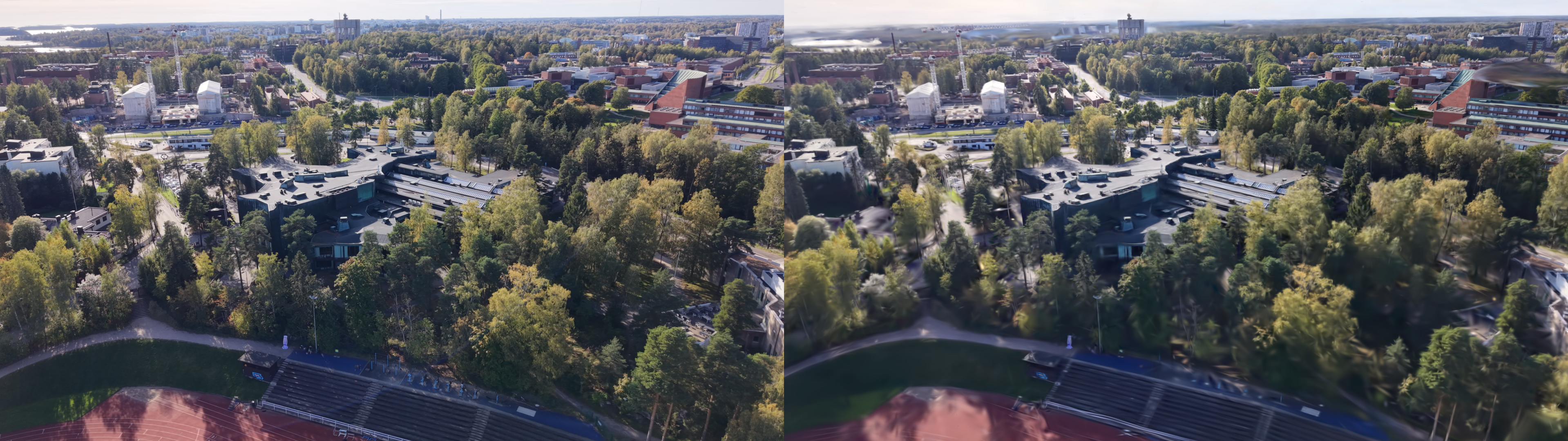
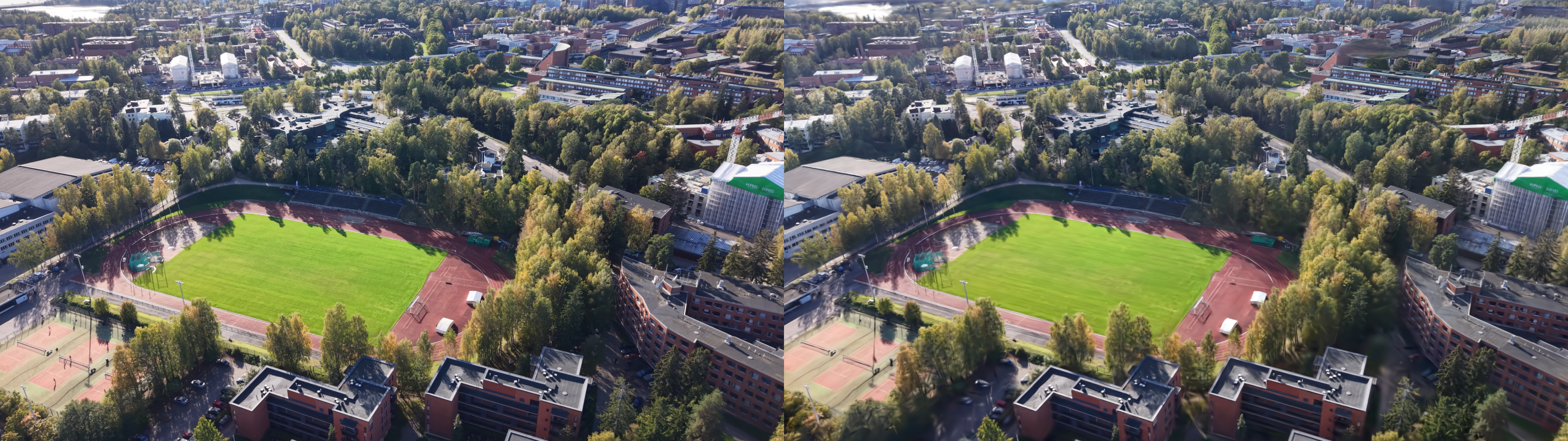
However, there are quite lots of floaters artifacts, some are hard to remove even with manual post-processing.

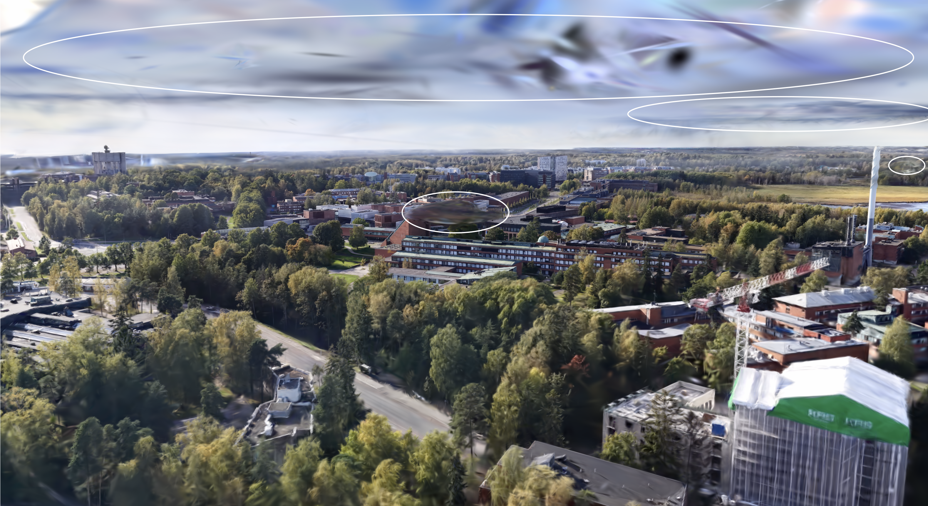
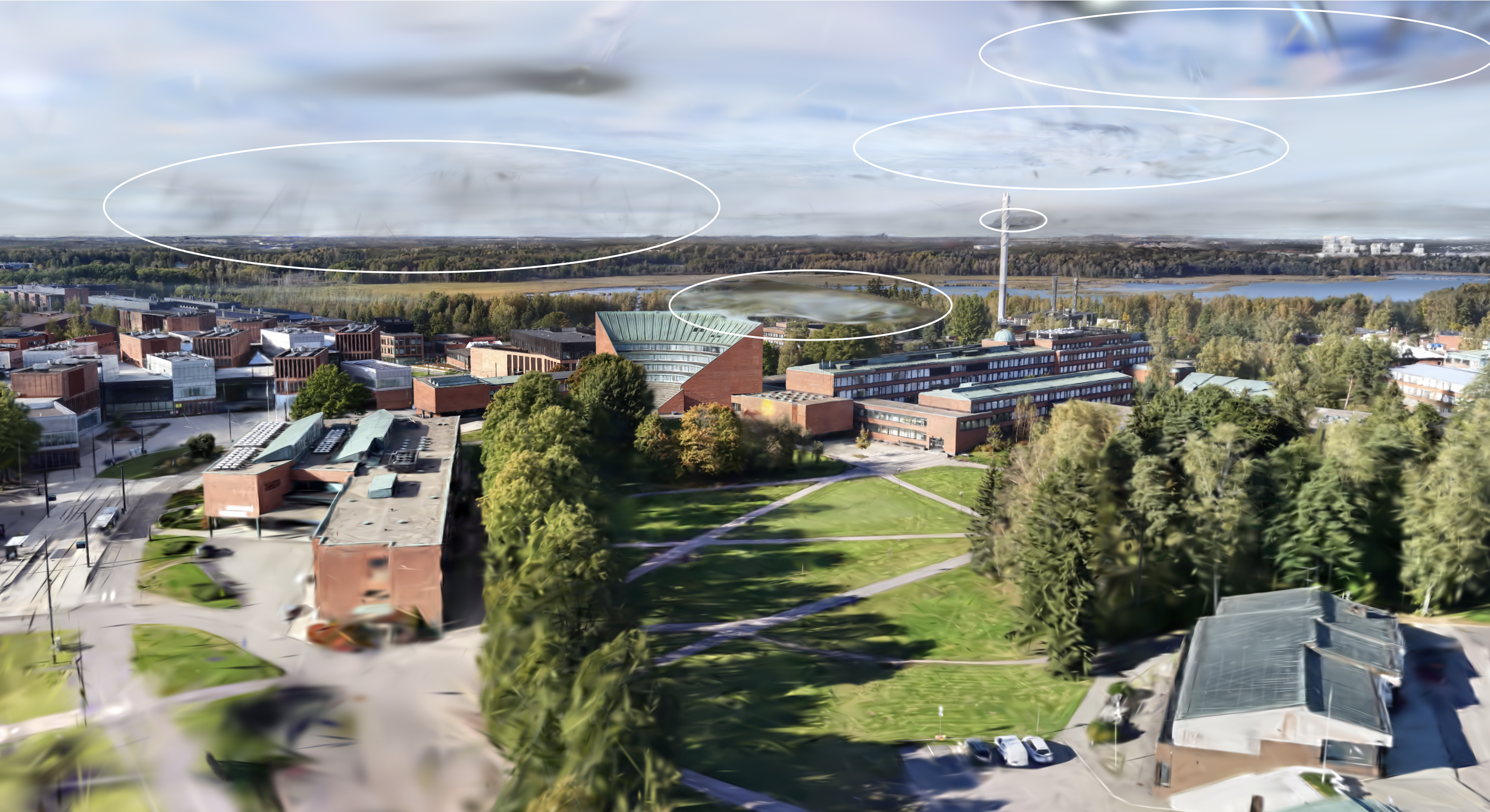
These floater artifacts are partly because 3DGS relies on carefully engineered heuristics for adaptive density control, with many parameters to tune e.g., opacity pruning threshold, image-plane gradient threshold for splitting/duplicating, 3D and 2D scale thresholds for pruning and splitting, reset interval, refinement interval, and more.. These heuristics also make 3DGS dependent on good initial point clouds, especially for real-world scenes, and make it non-trivial to estimate how many 3D Gaussians will be used for a given set of hyperparameters, making it difficult to control computation and memory budgets in advance.

3D Gaussian Splatting as Markov Chain Monte Carlo

To mitigate the problem above, I used 3DGS-MCMC by Kheradmand et al., which replaces the heuristic densification behavior in standard 3DGS with a relocation strategy motivated by an MCMC view.

For simplicity, consider the update of a single Gaussian $g_i$ in 3DGS, and momentarily ignore split/merge heuristics. Let $X=(g_1,\dots,g_N)$ denote the full set of Gaussians (the scene state). A standard gradient-based update on one Gaussian can be written as

where $\lambda_{\mathrm{lr}}$ is the learning rate, and $I$ is an image sampled from the training set $\mathcal{I}$.

Compare this to a typical SGLD-style block update:

where $\mathcal{P}(X)$ is the target density over scene configurations, and $\epsilon\sim \mathcal N(0,I)$ is Gaussian noise. These two equations become equivalent up to sign/scale conventions when $\lambda_{\mathrm{lr}}=-a$ and $b=0$.

This suggests that standard 3DGS optimization can be interpreted as a noise-free Langevin-style update on a component of the global scene state. Adding noise gives the SGLD-inspired form

Under this view, optimization in 3DGS over the full set of Gaussians can be seen as state transitions of a Markov chain: we move from one sample (a set of Gaussians) to another sample (a different configuration of Gaussians) This applies also to cases where the number of Gaussians changes, as one could think of the state with a smaller number of Gaussians simply as the equivalent state with more Gaussians, but with those that have zero opacity, that is, dead Gaussians., while relocation aims to keep successive states at similar probability (equivalently, similar rendering quality) so as not to disrupt the sampling dynamics.

To do state transition, 3DGS-MCMC do a simple strategy as moving ‘dead’ Gaussians to the location of ‘live’ Gaussians so that $P\left(X^{\text{new}}\right) \approx P\left(X^{\text{old}}\right)$. Specifically

To encourage Gaussians to disappear in non-useful locations and respawn, 3DGS-MCMC add regularization terms to opacity and covariance to the training loss:

There are several empirical implementation details (e.g., how to design the noise term to balance the gradient terms, only use noise for position not opacity, scale and color, learning rate, chosen values for regularization terms) that I will not cover here. For these, I recommend referring to the original paper.

Now running 3DGS-MCMC on our dataset, with 2M gaussians budget,many of the floater artifacts that were difficult to remove manually are eliminated automatically.The 3DGS-MCMC project page also shows similar results, where floater artifacts are significantly reduced compared to conventional 3DGS.

python3 simple_trainer.py mcmc \
  --data_dir ./data/aalto/ \
  --strategy.cap_max 2_000_000 \
  --data-factor 2 \
  --result-dir results/aalto/naive \
  --save-ply

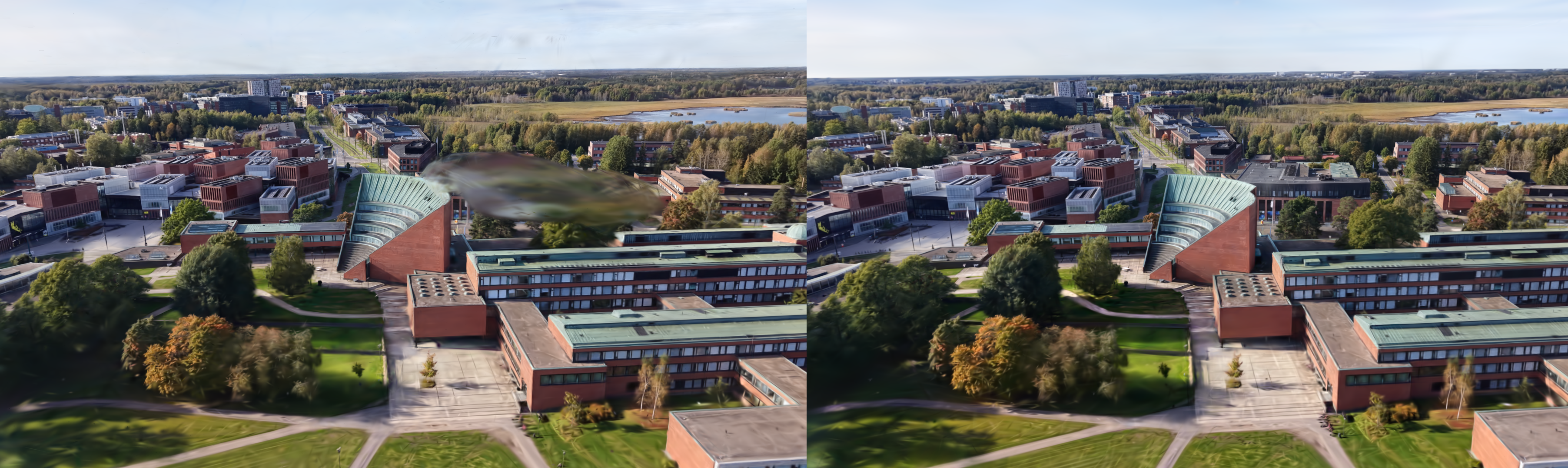
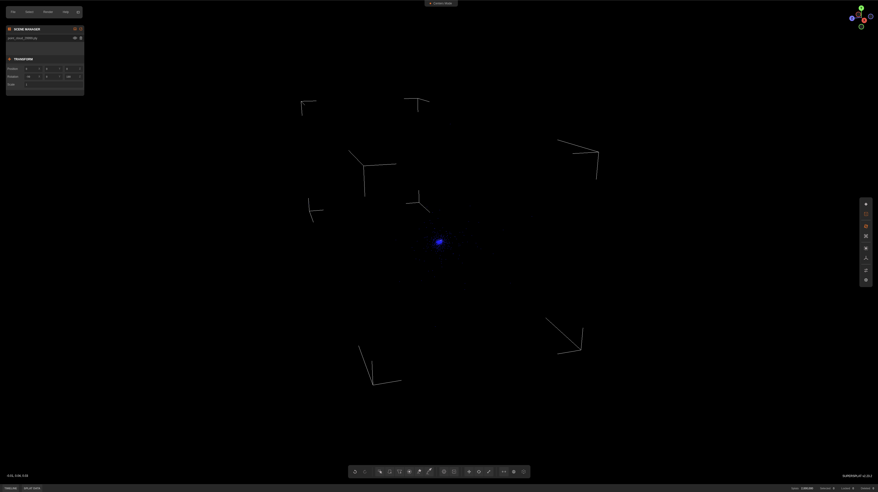
And the rest of the floaters can be removed with manual post-processing, in e.g superspt.at.

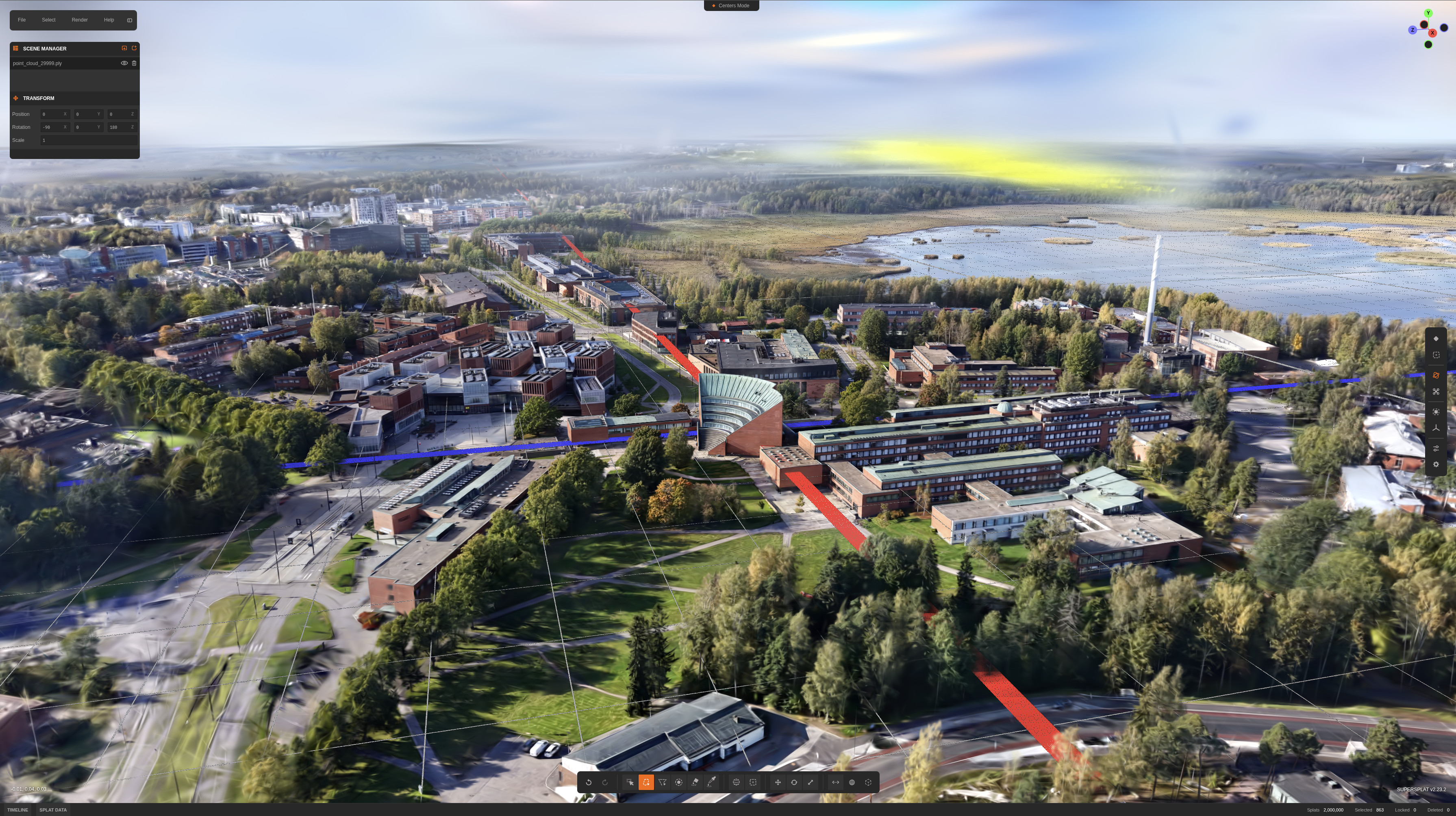
Note: though MCMC works great, it leads to very far-away Gaussians (see image), and makes the sorting system at runtime to sort Gaussians one galaxy away along with all the tiny Gaussians at the center of my scene (very inefficient). I just manually removed those post-processing.

Now we have a quite high fidelity scene representation using 2M gaussians. The .ply file is ~471.9MB in size (dependent on how many SH coefficients are used this will vary by a lot). Serving it on the web is kinda challening, since I want the scene to be downloaded and loaded instantly, so I need to compress it somehow. So let’s do that.

Compact 3D Scene Representation via Self-Organizing Gaussian Grids

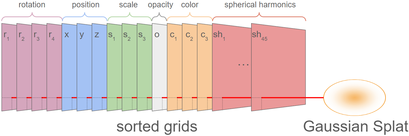
In standard 3DGS, scenes are stored as a flat list of Gaussians with their attributes in a .ply file. Each Gaussian carries 3 coordinates $(x, y, z)$, 3 scales $(s_x, s_y, s_z)$, 4 quaternion components $(q_x, q_y, q_z, q_w)$, 1 opacity $o$, 3 zeroth-order SH coefficients (base color), and $(L+1)^2$ SH coefficients for each additional degree $L$. That gives 14 attributes required to render a splat, plus 45 additional attributes for view-dependent effects (higher-order SH). For a scene with 2M Gaussians: $2\text{M} \times (14 + 45) \times 4\text{ bytes} \approx 471.9\text{ MB}$, which matches what we saw in the previous section.

There are various compression strategies to reduce this: keep only the top Gaussians by opacity, drop view-dependent effects by using only zeroth-order SH, quantize attributes to lower precision, and so on. Morgenstern et al. proposed Self-Organizing Gaussian Grids (SOGS), which takes a different approach: organize Gaussian parameters into 2D grids with local smoothness, then compress them as images.

The idea is to lay out each attribute, all X positions, all Y positions, each SH coefficient, as its own 2D image (59+ images for 59 attributes per Gaussian). Initially, these images look like random noise. SOGS then sorts the Gaussians within the grid so that neighbors share similar properties, transforming the noise into smooth, low-frequency images that compress dramatically better (e.g., 9x reduction for a sorted vs. random image with JPEG).

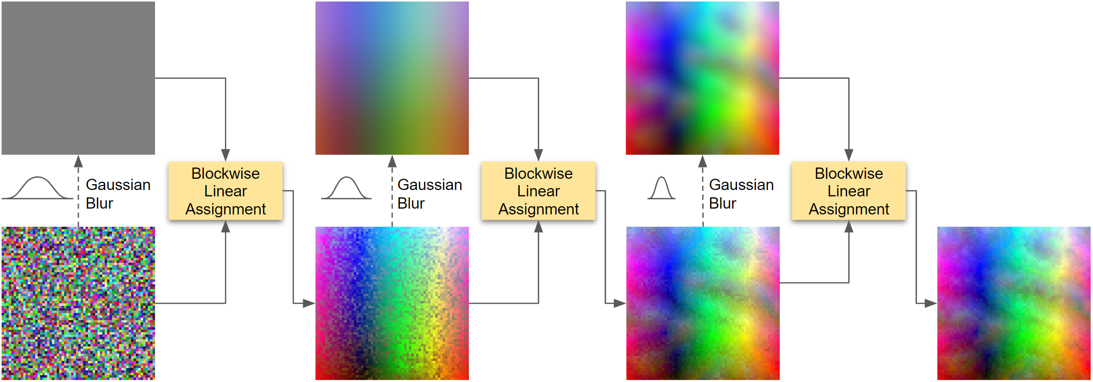
Parallel Linear Assignment Sorting (PLAS)

The sorting is done by PLAS, an iterative coarse-to-fine algorithm. Gaussians are first mapped to random grid positions to avoid local minima. At each iteration, a low-pass Gaussian filter (with radius $\varphi$) is applied to the current grid to produce a smooth target grid, and all elements are re-assigned to their best-matching positions in this target. The process repeats while decreasing the filter size, gradually refining the sort.

For each re-assignment step, the grid is divided into blocks of size $\beta = \varphi + 1$ (minimum $\beta = 16$ to maintain efficient parallelization), and each block is solved independently as a linear assignment problem. To sort across block boundaries, all blocks are shifted by a random $(\Delta x, \Delta y)$ before each re-assignment.

After each block-wise assignment, the mean $L_2$ distance between the sorted grid and target grid is measured. If the improvement drops below 0.01%, a new random block offset is tried. When the new offset also fails to improve beyond the threshold, the filter radius is reduced by $\varphi \leftarrow 0.95\,\varphi$, and the process continues at finer resolution.

By sorting on primary attributes (position, scale, base color), SOGS exploits the fact that Gaussians similar in these aspects also tend to have similar secondary attributes (opacity, rotation, higher-order SH). This “co-sorting” makes all attribute images smoother. Once sorted, standard 2D image compression codecs are applied to each attribute image.

To compress the scene post-training, I used the splat-transform library:

splat-transform aalto.ply aalto.sog

This produces a .sog file of 28.3 MB, a 16.7x reduction from the original 471.9 MB .ply.

Rendering on the Web

With the compressed .sog file, I wrote a browser-based 3D viewer to serve the scene as a static web application. The viewer is built on top of PlayCanvas engine, provides orbit, pan, fly, and zoom camera navigation, nine interactive location annotations with tooltips, ambient audio, fullscreen mode, and WebXR (AR/VR) entry points on supported devices. The source code is available at hoanhle/3d. You can see the runtime architecture and overview of the web viewer here.

Take-away

It took roughly 3 weeks: capturing the dataset, experimenting to get decent results and understanding each of the changes I made, serving it on the web, and all the tiny little things that go into making this project somewhat production-ready. It’s a fun project to work on, and I’m happy with the results. To reproduce the results now would take roughly a few hours.

Special Thanks

• Jaakko Lehtinen and Pauli Kemppinen for early comments and technical discussions.
• Aapo Pajunen for doing the drone captures with me.
• Donovan Hutchence of PlayCanvas for working with me to figure out how to render this scene nicely using their engine.
• Vincent Woo for inspiration on this project!